Today's subject
In the first post of the series we've looked at the CPython VM. We've learned that it works by executing a series of instructions called bytecode. We've also seen that Python bytecode is not sufficient to fully describe what a piece of code does. That's why there exists a notion of a code object. To execute a code block such as a module or a function means to execute a corresponding code object. A code object contains the block's bytecode, the constants and the names of variables used within the block and the block's various properties.
Typically, a Python programmer doesn't write bytecode and doesn't create the code objects but writes a normal Python code. So CPython must be able to create a code object from a source code. This job is done by the CPython compiler. In this part we'll explore how it works.
Note: In this post I'm referring to CPython 3.9. Some implementation details will certainly change as CPython evolves. I'll try to keep track of important changes and add update notes.
What the CPython compiler is
We understood what the responsibilities of the CPython compiler are, but before looking at how it is implemented, let's figure out why we call it a compiler in the first place.
A compiler, in its general sense, is a program that translates a program in one language into an equivalent program in another language. There are many types of compilers, but most of the time by a compiler we mean a static compiler, which translates a program in a high-level language to a machine code. Does the CPython compiler have something in common with this type of a compiler? To answer this question, let's take a look at the traditional three-stage design of a static compiler.
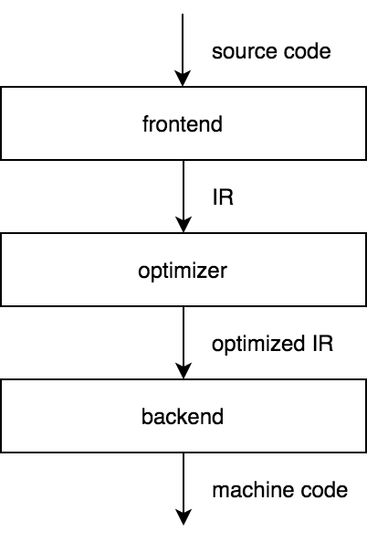
The frontend of a compiler transforms a source code into some intermediate representation (IR). The optimizer then takes an IR, optimizes it and passes an optimized IR to the backend that generates machine code. If we choose an IR that is not specific to any source language and any target machine, then we get a key benefit of the three-stage design: for a compiler to support a new source language, only an additional frontend is needed, and to support a new target machine, only an additional backend is needed.
The LLVM toolchain is a great example of a success of this model. There are frontends for C, Rust, Swift and many other programming languages that rely on LLVM to provide more complicated parts of the compiler. LLVM's creator, Chris Lattner, gives a good overview of its architecture.
CPython, however, doesn't need to support multiple source languages and target machines but only a Python code and the CPython VM. Nevertheless, the CPython compiler is an implementation of the three-stage design. To see why, we should examine the stages of a three-stage compiler in more detail.
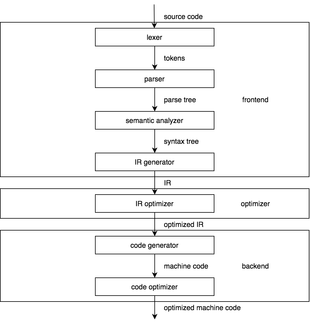
The picture above represents a model of a classic compiler. Now compare it to the architecture of the CPython compiler in the picture below.
Looks similar, doesn't it? The point here is that the structure of the CPython compiler should be familiar to anyone who studied compilers before. If you didn't, a famous Dragon Book is an excellent introduction to the theory of compiler construction. It's long, but you'll benefit even by reading only the first few chapters.
The comparison we've made requires several comments. First, since version 3.9, CPython uses a new parser by default that outputs an AST (Abstract Syntax Tree) straight away without an intermediate step of building a parse tree. Thus, the model of the CPython compiler is simplified even further. Second, some of the presented phases of the CPython compiler do so little compared to their counterparts of the static compilers that some may say that the CPython compiler is no more than a frontend. We won't take this view of the hardcore compiler writers.
Overview of the compiler's architecture
The diagrams are nice, but they hide many details and can be misleading, so let's spend some time discussing the overall design of the CPython compiler.
The two major components of the CPython compiler are:
- the frontend; and
- the backend.
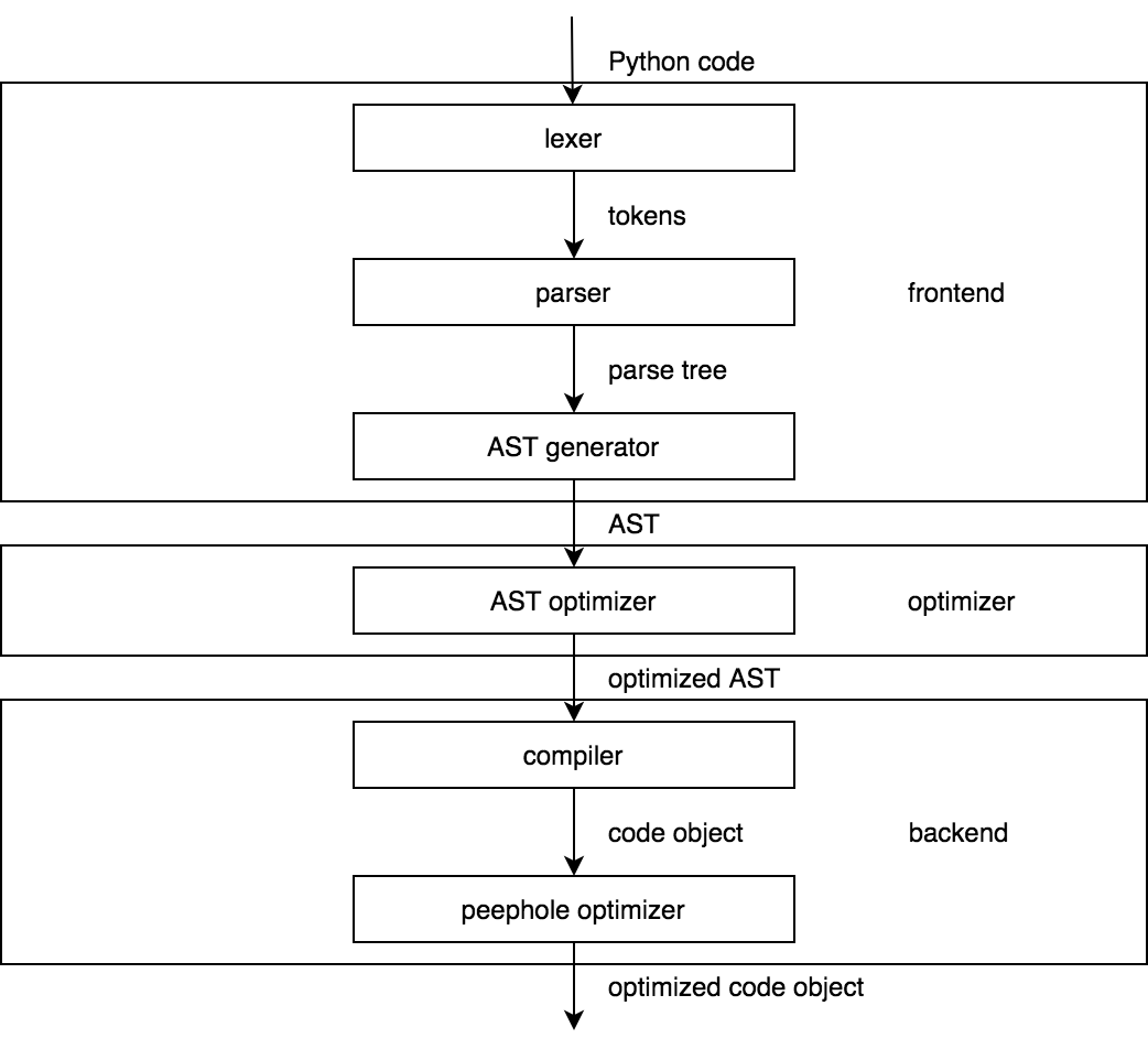
The frontend takes a Python code and produces an AST. The backend takes an AST and produces a code object. Throughout the CPython source code, the terms parser and compiler are used for the frontend and the backend respectively. This is yet another meaning of the word compiler. It was probably better to call it something like a code object generator, but we'll stick with the compiler since it doesn't seem to cause much trouble.
The job of the parser is to check whether the input is a syntactically correct Python code. If it's not, then the parser reports an error like the following:
x = y = = 12
        ^
SyntaxError: invalid syntax
If the input is correct, then the parser organizes it according to the rules of the grammar. A grammar defines the syntax of a language. The notion of a formal grammar is so crucial for our discussion that, I think, we should digress a little to recall its formal definition.
According to the classic definition, a grammar is a tuple of four items:
- \(\Sigma\) – a finite set of terminal symbols, or simply terminals (usually denoted by lowercase letters).
- \(N\) – a finite set of nonterminal symbols, or simply nonterminals (usually denoted by uppercase letters).
- \(P\) – a set of production rules. In the case of context-free grammars, which include the Python grammar, a production rule is just a mapping from a nonterminal to any sequence of terminals and nonterminals like \(A \to aB\).
- \(S\) – one distinguished nonterminal.
A grammar defines a language that consists of all sequences of terminals that can be generated by applying production rules. To generate some sequence, one starts with the symbol \(S\) and then recursively replaces each nonterminal with a sequence according to production rules until the whole sequence consists of terminals. Using established convention for the notation, it's sufficient to list production rules to specify the grammar. Here's, for example, a simple grammar that generates sequences of alternating ones and zeros:
\(S \to 10S \;| \;10\)
We'll continue to discuss grammars when we look at the parser in more detail.
Abstract syntax tree
The ultimate goal of the parser is to produce an AST. An AST is a tree data structure that serves as a high-level representation of a source code. Here's an example of a piece of code and a dump of the corresponding AST produced by the standard ast module:
x = 123
f(x)
$ python -m ast example1.py
Module(
   body=[
      Assign(
         targets=[
            Name(id='x', ctx=Store())],
         value=Constant(value=123)),
      Expr(
         value=Call(
            func=Name(id='f', ctx=Load()),
            args=[
               Name(id='x', ctx=Load())],
            keywords=[]))],
   type_ignores=[])
The types of the AST nodes are formally defined using the Zephyr Abstract Syntax Definition Language (ASDL). The ASDL is a simple declarative language that was created to describe tree-like IRs, which is what the AST is. Here's the definitions of the Assign and Expr nodes from Parser/Python.asdl:
stmt = ... | Assign(expr* targets, expr value, string? type_comment) | ...
expr = ... | Call(expr func, expr* args, keyword* keywords) | ...
The ASDL specification should give us an idea of what the Python AST looks like. The parser, however, needs to represent an AST in the C code. Fortunately, it's easy to generate the C structs for the AST nodes from their ASDL descriptions. That's what CPython does, and the result looks like this:
struct _stmt {
    enum _stmt_kind kind;
    union {
        // ... other kinds of statements
        struct {
            asdl_seq *targets;
            expr_ty value;
            string type_comment;
        } Assign;
        // ... other kinds of statements
    } v;
    int lineno;
    int col_offset;
    int end_lineno;
    int end_col_offset;
};

struct _expr {
    enum _expr_kind kind;
    union {
        // ... other kinds of expressions
        struct {
            expr_ty func;
            asdl_seq *args;
            asdl_seq *keywords;
        } Call;
        // ... other kinds of expressions
    } v;
    // ... same as in _stmt
};
An AST is a handy representation to work with. It tells what a program does, hiding all non-essential information such as indentation, punctuation and other Python's syntactic features.
One of the main beneficiaries of the AST representation is the compiler, which can walk an AST and emit bytecode in a relatively straightforward manner. Many Python tools, besides the compiler, use the AST to work with Python code. For example, pytest makes changes to an AST to provide useful information when the assert statement fails, which by itself does nothing but raises an AssertionError if the expression evaluates to False. Another example is Bandit that finds common security issues in Python code by analyzing an AST.
Now, when we've studied the Python AST a little bit, we can look at how the parser builds it from a source code.
From source code to AST
In fact, as I mentioned earlier, starting with version 3.9, CPython has not one but two parsers. The new parser is used by default. It's also possible to use the old parser by passing -X oldparser option. In CPython 3.10, however, the old parser will be completely removed.
The two parsers are very different. We'll focus on the new one, but before that, discuss the old parser as well.
old parser
For a long time Python's syntax was formally defined by the generative grammar. It's a kind of grammar we've talked about earlier. It tells us how to generate sequences belonging to the language. The problem is that a generative grammar doesn't directly correspond to the parsing algorithm that would be able to parse those sequences. Fortunately, smart people have been able to distinguish classes of generative grammars for which the corresponding parser can be built. These include context free, LL(k), LR(k), LALR and many other types of grammars. The Python grammar is LL(1). It's specified using a kind of Extended Backus–Naur Form (EBNF). To get an idea on how it can be used to describe Python's syntax, take a look at the rules for the while statement.
file_input: (NEWLINE | stmt)* ENDMARKER
stmt: simple_stmt | compound_stmt
compound_stmt: ... | while_stmt | ...
while_stmt: 'while' namedexpr_test ':' suite ['else' ':' suite]
suite: simple_stmt | NEWLINE INDENT stmt+ DEDENT
...
CPython extends the traditional notation with features like:
- grouping of alternatives: (a | b)
- optional parts: [a]
- zero or more and one or more repetitions: a* and a+.
We can see why Guido van Rossum chose to use regular expressions. They allow expressing the syntax of a programming language in a more natural (for a programmer) way. Instead of writing \(A \to aA | a\) , we can just write \(A \to a+\). This choice came with the cost: CPython had to develop a method to support the extended notation.
The parsing of an LL(1) grammar is a solved problem. The solution is a Pushdown Automaton (PDA) that acts as a top-down parser. A PDA operates by simulating the generation of an input string using a stack. To parse some input, it starts with the start symbol on the stack. Then it looks at the first symbol in the input, guesses which rule should be applied to the start symbol and replaces it with the right-hand side of that rule. If a top symbol on the stack is a terminal that matches the next symbol in the input, the PDA pops it and skips the matched symbol. If a top symbol is a nonterminal, the PDA tries to guess the rule to replace it with based on the next symbol in the input. The process repeats until the whole input is scanned or if the PDA can't match a terminal on the stack with the next symbol in the input. The latter case means that the input string cannot be parsed.
CPython couldn't use this method directly because of how the production rules are written, so the new method had to be developed. To support the extended notation, the old parser represents each rule of the grammar with a Deterministic Finite Automaton (DFA), which is famous for being equivalent to a regular expression. The parser itself is a stack-based automaton like PDA, but instead of pushing symbols on the stack, it pushes states of the DFAs. Here's the key data structures used by the old parser:
typedef struct {
    int              s_state;       /* State in current DFA */
    const dfa       *s_dfa;         /* Current DFA */
    struct _node    *s_parent;      /* Where to add next node */
} stackentry;

typedef struct {
    stackentry      *s_top;         /* Top entry */
    stackentry       s_base[MAXSTACK];/* Array of stack entries */
                                    /* NB The stack grows down */
} stack;

typedef struct {
    stack           p_stack;        /* Stack of parser states */
    grammar         *p_grammar;     /* Grammar to use */
                                    // basically, a collection of DFAs
    node            *p_tree;        /* Top of parse tree */
    // ...
} parser_state;
And the comment from Parser/parser.c that summarizes the approach:
A parsing rule is represented as a Deterministic Finite-state Automaton (DFA). A node in a DFA represents a state of the parser; an arc represents a transition. Transitions are either labeled with terminal symbols or with nonterminals. When the parser decides to follow an arc labeled with a nonterminal, it is invoked recursively with the DFA representing the parsing rule for that as its initial state; when that DFA accepts, the parser that invoked it continues. The parse tree constructed by the recursively called parser is inserted as a child in the current parse tree.
The parser builds a parse tree, also known as Concrete Syntax Tree (CST), while parsing an input. In contrast to an AST, a parse tree directly corresponds to the rules applied when deriving an input. All nodes in a parse tree are represented using the same node struct:
typedef struct _node {
    short               n_type;
    char                *n_str;
    int                 n_lineno;
    int                 n_col_offset;
    int                 n_nchildren;
    struct _node        *n_child;
    int                 n_end_lineno;
    int                 n_end_col_offset;
} node;
A parse tree, however, is not what the compiler waits for. It has to be converted to an AST. This work is done in Python/ast.c. The algorithm is to walk a parse tree recursively and translate its nodes to the AST nodes. Hardly anyone finds these nearly 6,000 lines of code exciting.
tokenizer
Python is not a simple language from the syntactic point of view. The Python grammar, though, looks simple and fits in about 200 lines including comments. This is because the symbols of the grammar are tokens and not individual characters. A token is represented by the type, such as NUMBER, NAME, NEWLINE, the value and the position in a source code. CPython distinguishes 63 types of tokens, all of which are listed in Grammar/Tokens. We can see what a tokenized program looks like using the standard tokenize module:
def x_plus(x):
    if x >= 0:
        return x
    return 0
$ python -m tokenize example2.py
0,0-0,0:            ENCODING       'utf-8'
1,0-1,3:            NAME           'def'
1,4-1,10:           NAME           'x_plus'
1,10-1,11:          OP             '('
1,11-1,12:          NAME           'x'
1,12-1,13:          OP             ')'
1,13-1,14:          OP             ':'
1,14-1,15:          NEWLINE        '\n'
2,0-2,4:            INDENT         '    '
2,4-2,6:            NAME           'if'
2,7-2,8:            NAME           'x'
2,9-2,11:           OP             '>='
2,12-2,13:          NUMBER         '0'
2,13-2,14:          OP             ':'
2,14-2,15:          NEWLINE        '\n'
3,0-3,8:            INDENT         '        '
3,8-3,14:           NAME           'return'
3,15-3,16:          NAME           'x'
3,16-3,17:          NEWLINE        '\n'
4,4-4,4:            DEDENT         ''
4,4-4,10:           NAME           'return'
4,11-4,12:          NUMBER         '0'
4,12-4,13:          NEWLINE        '\n'
5,0-5,0:            DEDENT         ''
5,0-5,0:            ENDMARKER      ''
This is how the program looks to the parser. When the parser needs a token, it requests one from the tokenizer. The tokenizer reads one character at a time from the buffer and tries to match the seen prefix with some type of token. How does the tokenizer work with different encodings? It relies on the io module. First, the tokenizer detects the encoding. If no encoding is specified, it defaults to UTF-8. Then, the tokenizer opens a file with a C call, which is equivalent to Python's open(fd, mode='r', encoding=enc), and reads its contents by calling the readline() function. This function returns a unicode string. The characters the tokenizer reads are just bytes in the UTF-8 representation of that string (or EOF).
We could define what a number or a name is directly in the grammar, though it would become more complex. What we couldn't do is to express the significance of indentation in the grammar without making it context-sensitive and, therefore, not suitable for parsing. The tokenizer makes the work of the parser much easier by providing the INDENT and DEDENT tokens. They mean what the curly braces mean in a language like C. The tokenizer is powerful enough to handle indentation because it has state. The current indentation level is kept on the top of the stack. When the level is increased, it's pushed on the stack. If the level is decreased, all higher levels are popped from the stack.
The old parser is a non-trivial piece of the CPython codebase. The DFAs for the rules of the grammar are generated automatically, but other parts of the parser are written by hand. This is in contrast with the new parser, which seems to be a much more elegant solution to the problem of parsing Python code.
new parser
The new parser comes with the new grammar. This grammar is a Parsing Expression Grammar (PEG). The important thing to understand is that PEG is not just a class of grammars. It's another way to define a grammar. PEGs were introduced by Bryan Ford in 2004 as a tool to describe a programming language and to generate a parser based on the description. A PEG is different from the traditional formal grammar in that its rules map nonterminals to the parsing expressions instead of just sequences of symbols. This is in the spirit of CPython. A parsing expression is defined inductively. If \(e\), \(e_1\), and \(e_2\) are parsing expressions, then so is:
- the empty string
- any terminal
- any nonterminal
- \(e_1e_2\), a sequence
- \(e_1/e_2\), prioritized choice
- \(e*\), zero-or-more repetitions
- \(!e\), a not-predicate.
PEGs are analytic grammars, which means that they are designed not only to generate languages but to analyze them as well. Ford formalized what it means for a parsing expression \(e\) to recognize an input \(x\). Basically, any attempt to recognize an input with some parsing expression can either succeed or fail and consume some input or not. For example, applying the parsing expression \(a\) to the input \(ab\) results in a success and consumes \(a\).
This formalization allows converting any PEG to a recursive descent parser. A recursive descent parser associates each nonterminal of a grammar with a parsing function. In the case of a PEG, the body of a parsing function is an implementation of the corresponding parsing expression. If a parsing expression contains nonterminals, their parsing functions are called recursively.
A nonterminal may have multiple production rules. A recursive descent parser has to decide which one was used to derive the input. If a grammar is LL(k), a parser can look at the next k tokens in the input and predict the correct rule. Such a parser is called a predictive parser. If it's not possible to predict, the backtracking method is used. A parser with backtracking tries one rule, and, if fails, backtracks and tries another. This is exactly what the prioritized choice operator in a PEG does. So, a PEG parser is a recursive descent parser with backtracking.
The backtracking method is powerful but can be computationally costly. Consider a simple example. We apply the expression \(AB/A\) to the input that succeeds on \(A\) but then fails on \(B\). According to the the interpretation of the prioritized choice operator, the parser first tries to recognize \(A\), succeeds, and then tries to recognize B. It fails on \(B\) and tries to recognize \(A\) again. Because of such redundant computations, the parse time can be exponential in the size of the input. To remedy this problem, Ford suggested to use a memoization technique, i.e. caching the results of function calls. Using this technique, the parser, known as the packrat parser, is guaranteed to work in linear time at the expense of a higher memory consumption. And this is what CPython's new parser does. It's a packrat parser!
No matter how good the new parser is, the reasons to replace the old parser have to be given. This is what the PEPs are for. PEP 617 -- New PEG parser for CPython gives a background on both the old and the new parser and explains the reasons behind the transition. In a nutshell, the new parser removes the LL(1) restriction on the grammar and should be easier to maintain. Guido van Rossum wrote an excellent series on a PEG parsing, in which he goes into much more detail and shows how to implement a simple PEG parser. We, in our turn, will take a look at its CPython implementation.
You might be surprised to learn that the new grammar file is more than three times bigger than the old one. This is because the new grammar is not just a grammar but a Syntax-Directed Translation Scheme (SDTS). An SDTS is a grammar with actions attached to the rules. An action is a piece of code. A parser executes an action when it applies the corresponding rule to the input and succeeds. CPython uses actions to build an AST while parsing. To see how, let's see what the new grammar looks like. We've already seen the rules of the old grammar for the while statement, so here's their new analogues:
file[mod_ty]: a=[statements] ENDMARKER { _PyPegen_make_module(p, a) }
statements[asdl_seq*]: a=statement+ { _PyPegen_seq_flatten(p, a) }
statement[asdl_seq*]: a=compound_stmt { _PyPegen_singleton_seq(p, a) } | simple_stmt
compound_stmt[stmt_ty]:
    | ...
    | &'while' while_stmt
while_stmt[stmt_ty]:
    | 'while' a=named_expression ':' b=block c=[else_block] { _Py_While(a, b, c, EXTRA) }
...
Each rule starts with the name of a nonterminal. It's followed by the C type of the result that the parsing function returns. The right-hand side is a parsing expression. The code in the curly braces denotes an action. Actions are simple function calls that return AST nodes or their fields.
The new parser is Parser/pegen/parse.c. It's generated automatically by the parser generator. The parser generator is written in Python. It's a program that takes a grammar and generates a PEG parser in C or Python. A grammar is described in the grammar file and represented by the instance of the Grammar class. To create such an instance, there must be a parser for the grammar file. This parser is also generated automatically by the parser generator from the metagrammar. That's why the parser generator can generate a parser in Python. But what parses the metagrammar? Well, it's in the same notation as grammar, so the generated grammar parser is able to parse the metagrammar as well. Of course, the grammar parser had to be bootstrapped, i.e. the first version had to be written by hand. Once that's done, all parsers can be generated automatically.
Like the old parser, the new parser gets tokens from the tokenizer. This is unusual for a PEG parser since it allows unifying tokenization and parsing. But we saw that the tokenizer does a non-trivial job, so the CPython developers decided to make use of it.
On this note, we end our discussion of parsing to see what happens next to an AST.
AST optimization
The diagram of the CPython compiler's architecture shows us the AST optimizer alongside the parser and the compiler. This probably overemphasizes the optimizer's role. The AST optimizer is confined to constant folding and was introduced only in CPython 3.7. Before CPython 3.7, constant folding was done at a later stage by the peephole optimizer. Nonetheless, due to the AST optimizer, we can write things like this:
n = 2 ** 32 # easier to write and to read
and expect it to be calculated at compile time.
An example of a less obvious optimization is the conversion of a list of constants and a set of constants into a tuple and a frozenset respectively. This optimization is performed when a list or a set are used on the right-hand side of the in or not in operators.
From AST to code object
Up until now, we've been studying how CPython creates an AST from a source code, but as we've seen in the first post, the CPython VM knows nothing about the AST and is only able to execute a code object. The conversion of an AST to a code object is a job of the compiler. More specifically, the compiler must return the module's code object containing the module's bytecode along with the code objects for other code blocks in the module such as defined functions and classes.
Sometimes the best way to understand a solution to a problem is to think of one's own. Let's ponder what we would do if we were the compiler. We start with the root node of an AST that represents a module. Children of this node are statements. Let's assume that the first statement is a simple assignment like x = 1. It's represented by the Assign AST node: Assign(targets=[Name(id='x', ctx=Store())], value=Constant(value=1)). To convert this node to a code object we need to create one, store constant 1 in the list of constants of the code object, store the name of the variable x in the list of names used in the code object and emit the LOAD_CONST and STORE_NAME instructions. We could write a function to do that. But even a simple assignment can be tricky. For example, imagine that the same assignment is made inside the body of a function. If x is a local variable, we should emit the STORE_FAST instruction. If x is a global variable, we should emit the STORE_GLOBAL instruction. Finally, if x is referenced by a nested function, we should emit the STORE_DEREF instruction. The problem is to determine what the type of the variable x is. CPython solves this problem by building a symbol table before compiling.
symbol table
A symbol table contains information about code blocks and the symbols used within them. It's represented by a single symtable struct and a collection of _symtable_entry structs, one for each code block in a program. A symbol table entry contains the properties of a code block, including its name, its type (module, class or function) and a dictionary that maps the names of variables used within the block to the flags indicating their scope and usage. Here's the complete definition of the _symtable_entry struct:
typedef struct _symtable_entry {
    PyObject_HEAD
    PyObject *ste_id;        /* int: key in ste_table->st_blocks */
    PyObject *ste_symbols;   /* dict: variable names to flags */
    PyObject *ste_name;      /* string: name of current block */
    PyObject *ste_varnames;  /* list of function parameters */
    PyObject *ste_children;  /* list of child blocks */
    PyObject *ste_directives;/* locations of global and nonlocal statements */
    _Py_block_ty ste_type;   /* module, class, or function */
    int ste_nested;      /* true if block is nested */
    unsigned ste_free : 1;        /* true if block has free variables */
    unsigned ste_child_free : 1;  /* true if a child block has free vars,
                                     including free refs to globals */
    unsigned ste_generator : 1;   /* true if namespace is a generator */
    unsigned ste_coroutine : 1;   /* true if namespace is a coroutine */
    unsigned ste_comprehension : 1; /* true if namespace is a list comprehension */
    unsigned ste_varargs : 1;     /* true if block has varargs */
    unsigned ste_varkeywords : 1; /* true if block has varkeywords */
    unsigned ste_returns_value : 1;  /* true if namespace uses return with
                                        an argument */
    unsigned ste_needs_class_closure : 1; /* for class scopes, true if a
                                             closure over __class__
                                             should be created */
    unsigned ste_comp_iter_target : 1; /* true if visiting comprehension target */
    int ste_comp_iter_expr; /* non-zero if visiting a comprehension range expression */
    int ste_lineno;          /* first line of block */
    int ste_col_offset;      /* offset of first line of block */
    int ste_opt_lineno;      /* lineno of last exec or import * */
    int ste_opt_col_offset;  /* offset of last exec or import * */
    struct symtable *ste_table;
} PySTEntryObject;
CPython uses the term namespace as a synonym for a code block in the context of symbol tables. So, we can say that a symbol table entry is a description of a namespace. The symbol table entries form an hierarchy of all namespaces in a program through the ste_children field, which is a list of child namespaces. We can explore this hierarchy using the standard symtable module:
# example3.py
def func(x):
    lc = [x+i for i in range(10)]
    return lc
>>> from symtable import symtable
>>> f = open('example3.py')
>>> st = symtable(f.read(), 'example3.py', 'exec') # module's symtable entry
>>> dir(st)
[..., 'get_children', 'get_id', 'get_identifiers', 'get_lineno', 'get_name',
 'get_symbols', 'get_type', 'has_children', 'is_nested', 'is_optimized', 'lookup']
>>> st.get_children()
[<Function SymbolTable for func in example3.py>]
>>> func_st = st.get_children()[0] # func's symtable entry
>>> func_st.get_children()
[<Function SymbolTable for listcomp in example3.py>]
>>> lc_st = func_st.get_children()[0] # list comprehension's symtable entry
>>> lc_st.get_symbols()
[<symbol '.0'>, <symbol 'i'>, <symbol 'x'>]
>>> x_sym = lc_st.get_symbols()[2]
>>> dir(x_sym)
[..., 'get_name', 'get_namespace', 'get_namespaces', 'is_annotated',
 'is_assigned', 'is_declared_global', 'is_free', 'is_global', 'is_imported',
 'is_local', 'is_namespace', 'is_nonlocal', 'is_parameter', 'is_referenced']
>>> x_sym.is_local(), x_sym.is_free()
(False, True)
This example shows that every code block has a corresponding symbol table entry. We've accidentally come across the strange .0 symbol inside the namespace of the list comprehension. This namespace doesn't contain the range symbol, which is also strange. This is because a list comprehension is implemented as an anonymous function and range(10) is passed to it as an argument. This argument is referred to as .0. What else does CPython hide from us?
The symbol table entries are constructed in two passes. During the first pass, CPython walks the AST and creates a symbol table entry for each code block it encounters. It also collects information that can be collected on the spot, such as whether a symbol is defined or used in the block. But some information is hard to deduce during the first pass. Consider the example:
def top():
    def nested():
        return x + 1
    x = 10
    ...
When constructing a symbol table entry for the nested() function, we cannot tell whether x is a global variable or a free variable, i.e. defined in the top() function, because we haven't seen an assignment yet.
CPython solves this problem by doing the second pass. At the start of the second pass it's already known where the symbols are defined and used. The missing information is filled by visiting recursively all the symbol table entries starting from the top. The symbols defined in the enclosing scope are passed down to the nested namespace, and the names of free variables in the enclosed scope are passed back.
The symbol table entries are managed using the symtable struct. It's used both to construct the symbol table entries and to access them during the compilation. Let's take a look at its definition:
struct symtable {
    PyObject *st_filename;          /* name of file being compiled,
                                       decoded from the filesystem encoding */
    struct _symtable_entry *st_cur; /* current symbol table entry */
    struct _symtable_entry *st_top; /* symbol table entry for module */
    PyObject *st_blocks;            /* dict: map AST node addresses
                                     *       to symbol table entries */
    PyObject *st_stack;             /* list: stack of namespace info */
    PyObject *st_global;            /* borrowed ref to st_top->ste_symbols */
    int st_nblocks;                 /* number of blocks used. kept for
                                       consistency with the corresponding
                                       compiler structure */
    PyObject *st_private;           /* name of current class or NULL */
    PyFutureFeatures *st_future;    /* module's future features that affect
                                       the symbol table */
    int recursion_depth;            /* current recursion depth */
    int recursion_limit;            /* recursion limit */
};
The most important fields to note are st_stack and st_blocks. The st_stack field is a stack of symbol table entries. During the first pass of the symbol table construction, CPython pushes an entry onto the stack when it enters the corresponding code block and pops an entry from the stack when it exits the corresponding code block. The st_blocks field is a dictionary that the compiler uses to get a symbol table entry for a given AST node. The st_cur and st_top fields are also important but their meanings should be obvious.
To learn more about symbol tables and their construction, I highly recommend you the articles by Eli Bendersky.
basic blocks
A symbol table helps us to translate statements involving variables like x = 1. But a new problem arises if we try to translate a more complex control-flow statement. Consider another cryptic piece of code:
if x == 0 or x > 17:
    y = True
else:
    y = False
...
The corresponding AST subtree has the following structure:
If(
  test=BoolOp(...),
  body=[...],
  orelse=[...]
)
And the compiler translates it to the following bytecode:
1           0 LOAD_NAME                0 (x)
            2 LOAD_CONST               0 (0)
            4 COMPARE_OP               2 (==)
            6 POP_JUMP_IF_TRUE        16
            8 LOAD_NAME                0 (x)
           10 LOAD_CONST               1 (17)
           12 COMPARE_OP               4 (>)
           14 POP_JUMP_IF_FALSE       22

2     >>   16 LOAD_CONST               2 (True)
           18 STORE_NAME               1 (y)
           20 JUMP_FORWARD             4 (to 26)

4     >>   22 LOAD_CONST               3 (False)
           24 STORE_NAME               1 (y)
5     >>   26 ...
The bytecode is linear. The instructions for the test node should come first, and the instructions for the body block should come before those for the orelse block. The problem with the control-flow statements is that they involve jumps, and a jump is often emitted before the instruction it points to. In our example, if the first test succeeds, we would like to jump to the first body instruction straight away, but we don't know where it should be yet. If the second test fails, we have to jump over the body block to the orelse block, but the position of the first orelse instruction will become known only after we translate the body block.
We could solve this problem if we move the instructions for each block into a separate data structure. Then, instead of specifying jump targets as concrete positions in the bytecode, we point to those data structures. Finally, when all blocks are translated and their sizes are know, we calculate arguments for jumps and assemble the blocks into a single sequence of instructions. And that's what the compiler does.
The blocks we're talking about are called basic blocks. They are not specific to CPython, though CPython's notion of a basic block differs from the conventional definition. According to the Dragon book, a basic block is a maximal sequence of instructions such that:
-
control may enter only the first instruction of the block; and
-
control will leave the block without halting or branching, except possibly at the last instruction.
CPython drops the second requirement. In other words, no instruction of a basic block except the first can be a target of a jump, but a basic block itself can contain jump instructions. To translate the AST from our example, the compiler creates four basic blocks:
- instructions 0-14 for
test - instructions 16-20 for
body - instructions 22-24 for
orelse; and - instructions 26-... for whatever comes after the if statement.
A basic block is represented by the basicblock_ struct that is defined as follows:
typedef struct basicblock_ {
    /* Each basicblock in a compilation unit is linked via b_list in the
       reverse order that the block are allocated.  b_list points to the next
       block, not to be confused with b_next, which is next by control flow. */
    struct basicblock_ *b_list;
    /* number of instructions used */
    int b_iused;
    /* length of instruction array (b_instr) */
    int b_ialloc;
    /* pointer to an array of instructions, initially NULL */
    struct instr *b_instr;
    /* If b_next is non-NULL, it is a pointer to the next
       block reached by normal control flow. */
    struct basicblock_ *b_next;
    /* b_seen is used to perform a DFS of basicblocks. */
    unsigned b_seen : 1;
    /* b_return is true if a RETURN_VALUE opcode is inserted. */
    unsigned b_return : 1;
    /* depth of stack upon entry of block, computed by stackdepth() */
    int b_startdepth;
    /* instruction offset for block, computed by assemble_jump_offsets() */
    int b_offset;
} basicblock;
And here's the definition of the instr struct:
struct instr {
    unsigned i_jabs : 1;
    unsigned i_jrel : 1;
    unsigned char i_opcode;
    int i_oparg;
    struct basicblock_ *i_target; /* target block (if jump instruction) */
    int i_lineno;
};
We can see that the basic blocks are connected not only by jump instructions but also through the b_list and b_next fields. The compiler uses b_list to access all allocated blocks, for example, to free the memory. The b_next field is of more interest to us right now. As the comment says, it points to the next block reached by the normal control flow, which means that it can be used to assemble blocks in the right order. Returning to our example once more, the test block points to the body block, the body block points to the orelse block and the orelse block points to the block after the if statement. Because basic blocks point to each other, they form a graph called a Control Flow Graph (CFG).
frame blocks
There is one more problem to solve: how to understand where to jump to when compiling statements like continue and break? The compiler solves this problem by introducing yet another type of block called frame block. There are different kinds of frame blocks. The WHILE_LOOP frame block, for example, points to two basic blocks: the body block and the block after the while statement. These basic blocks are used when compiling the continue and break statements respectively. Since frame blocks can nest, the compiler keeps track of them using stacks, one stack of frame blocks per code block. Frame blocks are also useful when dealing with statements such as try-except-finally, but we will not dwell on this now. Let's instead have a look at the definition of the fblockinfo struct:
enum fblocktype { WHILE_LOOP, FOR_LOOP, EXCEPT, FINALLY_TRY, FINALLY_END,
                  WITH, ASYNC_WITH, HANDLER_CLEANUP, POP_VALUE };

struct fblockinfo {
    enum fblocktype fb_type;
    basicblock *fb_block;
    /* (optional) type-specific exit or cleanup block */
    basicblock *fb_exit;
    /* (optional) additional information required for unwinding */
    void *fb_datum;
};
We've identified three important problems and we've seen how the compiler solves them. Now, let's put everything together to see how the compiler works from the beginning to the end.
compiler units, compiler and assembler
As we've already figured out, after building a symbol table, the compiler performs two more steps to convert an AST to a code object:
- it creates a CFG of basic blocks; and
- it assembles a CFG into a code object.
This two-step process is performed for each code block in a program. The compiler starts by building the module's CFG and ends by assembling the module's CFG into the module's code object. In between, it walks the AST by recursively calling the compiler_visit_* and compiler_* functions, where * denotes what is visited or compiled. For example, compiler_visit_stmt delegates the compilation of a given statement to the appropriate compiler_* function, and the compiler_if function knows how to compile the If AST node. If a node introduces new basic blocks, the compiler creates them. If a node begins a code block, the compiler creates a new compilation unit and enters it. A compilation unit is a data structure that captures the compilation state of the code block. It acts as a mutable prototype of the code object and points to a new CFG. The compiler assembles this CFG when it exits a node that began the current code block. The assembled code object is stored in the parent compilation unit. As always, I encourage you to look at the struct definition:
struct compiler_unit {
    PySTEntryObject *u_ste;

    PyObject *u_name;
    PyObject *u_qualname;  /* dot-separated qualified name (lazy) */
    int u_scope_type;

    /* The following fields are dicts that map objects to
       the index of them in co_XXX.      The index is used as
       the argument for opcodes that refer to those collections.
    */
    PyObject *u_consts;    /* all constants */
    PyObject *u_names;     /* all names */
    PyObject *u_varnames;  /* local variables */
    PyObject *u_cellvars;  /* cell variables */
    PyObject *u_freevars;  /* free variables */

    PyObject *u_private;        /* for private name mangling */

    Py_ssize_t u_argcount;        /* number of arguments for block */
    Py_ssize_t u_posonlyargcount;        /* number of positional only arguments for block */
    Py_ssize_t u_kwonlyargcount; /* number of keyword only arguments for block */
    /* Pointer to the most recently allocated block.  By following b_list
       members, you can reach all early allocated blocks. */
    basicblock *u_blocks;
    basicblock *u_curblock; /* pointer to current block */

    int u_nfblocks;
    struct fblockinfo u_fblock[CO_MAXBLOCKS];

    int u_firstlineno; /* the first lineno of the block */
    int u_lineno;          /* the lineno for the current stmt */
    int u_col_offset;      /* the offset of the current stmt */
};
Another data structure that is crucial for the compilation is the compiler struct, which represents the global state of the compilation. Here's its definition:
struct compiler {
    PyObject *c_filename;
    struct symtable *c_st;
    PyFutureFeatures *c_future; /* pointer to module's __future__ */
    PyCompilerFlags *c_flags;

    int c_optimize;              /* optimization level */
    int c_interactive;           /* true if in interactive mode */
    int c_nestlevel;
    int c_do_not_emit_bytecode;  /* The compiler won't emit any bytecode
                                    if this value is different from zero.
                                    This can be used to temporarily visit
                                    nodes without emitting bytecode to
                                    check only errors. */

    PyObject *c_const_cache;     /* Python dict holding all constants,
                                    including names tuple */
    struct compiler_unit *u; /* compiler state for current block */
    PyObject *c_stack;           /* Python list holding compiler_unit ptrs */
    PyArena *c_arena;            /* pointer to memory allocation arena */
};
And the comment preceding the definition that explains what the two most important fields are for:
The u pointer points to the current compilation unit, while units for enclosing blocks are stored in c_stack. The u and c_stack are managed by compiler_enter_scope() and compiler_exit_scope().
To assemble basic blocks into a code object, the compiler first has to fix the jump instructions by replacing pointers with positions in bytecode. On the one side, it's an easy task, since the sizes of all basic blocks are known. On the other side, the size of a basic block can change when we fix a jump. The current solution is to keep fixing jumps in a loop while the sizes change. Here's an honest comment from the source code on this solution:
This is an awful hack that could hurt performance, but on the bright side it should work until we come up with a better solution.
The rest is straightforward. The compiler iterates over basic blocks and emits the instructions. The progress is kept in the assembler struct:
struct assembler {
    PyObject *a_bytecode;  /* string containing bytecode */
    int a_offset;              /* offset into bytecode */
    int a_nblocks;             /* number of reachable blocks */
    basicblock **a_postorder; /* list of blocks in dfs postorder */
    PyObject *a_lnotab;    /* string containing lnotab */
    int a_lnotab_off;      /* offset into lnotab */
    int a_lineno;              /* last lineno of emitted instruction */
    int a_lineno_off;      /* bytecode offset of last lineno */
};
At this point, the current compilation unit and the assembler contain all the data needed to create a code object. Congratulations! We've done it! Almost.
peephole optimizer
The last step in the creation of the code object is to optimize the bytecode. This is a job of the peephole optimizer. Here's some types of optimizations it performs:
- The statements like
if True: ...andwhile True: ...generate a sequence ofLOAD_CONST trueconstandPOP_JUMP_IF_FALSEinstructions. The peephole optimizer eliminates such instructions. - The statements like
a, = b,lead to the bytecode that builds a tuple and then unpacks it. The peephole optimizer replaces it with a simple assignment. - The peephole optimizer removes unreachable instructions after
RETURN.
Essentially, the peephole optimizer removes redundant instructions, thus making bytecode more compact. After the bytecode is optimized, the compiler creates the code object, and the VM is ready to execute it.
Summary
This was a long post, so it's probably a good idea to sum up what we've learned. The architecture of the CPython compiler follows a traditional design. Its two major parts are the frontend and the backend. The frontend is also referred to as the parser. Its job is to convert a source code to an AST. The parser gets tokens from the tokenizer, which is responsible for producing a stream of meaningful language units from the text. Historically, the parsing consisted of several steps, including the generation of a parse tree and the conversion of a parse tree to an AST. In CPython 3.9, the new parser was introduced. It's based on a parsing expression grammar and produces an AST straight away. The backend, also known paradoxically as the compiler, takes an AST and produces a code object. It does this by first building a symbol table and then by creating one more intermediate representation of a program called a control flow graph. The CFG is assembled into a single sequence of instructions, which is then optimized by the peephole optimizer. Eventually, the code object gets created.
At this point, we have enough knowledge to get acquainted with the CPython source code and understand some of the things it does. That's our plan for the next time.
If you have any questions, comments or suggestions, feel free to contact me at victor@tenthousandmeters.com
Follow me for more content: GitHub | Bluesky | Twitter | LinkedIn